a)
Write a code which simulates Conway's Game of Life on a \(20\times20\) grid with periodic boundary conditions.
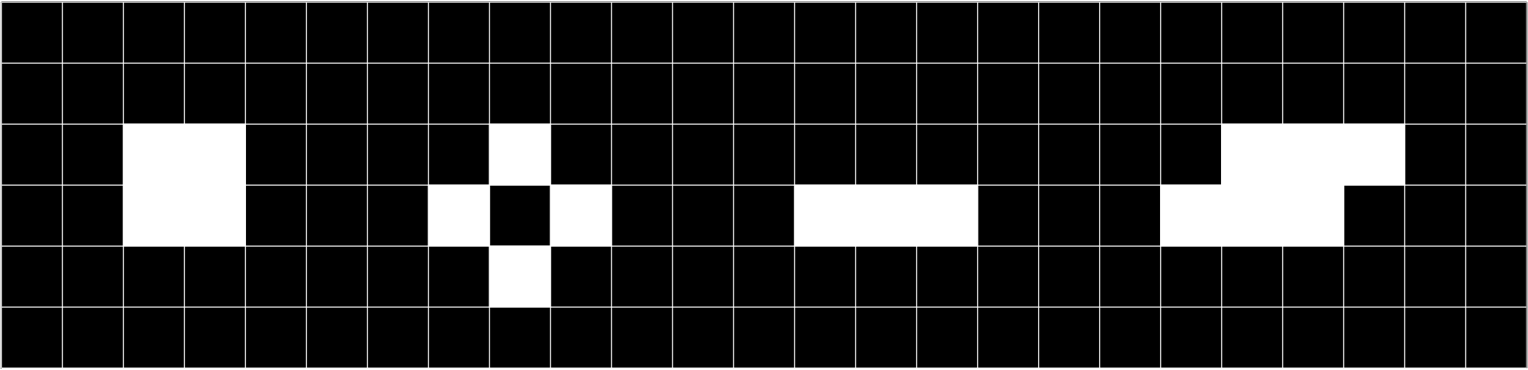
Check your code with a few simple configurations, such as the ones shown in the figure:
rule30(). This function will first define the rule as a
\(2\times2\times2\) look up table rule.
rule = cat([0 1; 1 0], [1 1; 0 0], dims=3)
evol, which will be used to store the evolution of the values of all
\(120\) cells (columns) over all time steps (rows). We will initialize the values as 0 (using Julia's build in function zeros([T=Int64,] dims...)),
which is convenient because we want to set the value of most cells in the start configuration to \(0\).
evol = zeros(Int64,51,120)
evol[1,60]=1
rule
(\(+1\) for Julia convention).
        for g in 2:51
          for i in 1:120
            evol[g,i]= rule[evol[g-1,mod1(i-1,120)]+1,evol[g-1,i]+1,evol[g-1,mod1(i+1,120)]+1]
          end
        end
mod1(x,m) function (with \(m=120\)).evol.rule30() looks like this
        function rule30()
          rule = cat([0 1; 1 0], [1 1; 0 0], dims=3)
          evol = zeros(Int64,51,120)
          evol[1,60]=1
          for g in 2:51
            for i in 1:120
              evol[g,i]= rule[evol[g-1,mod1(i-1,120)]+1,evol[g-1,i]+1,evol[g-1,mod1(i+1,120)]+1]
            end
          end
          return evol
        end
evol matrix, which can in Julia easily be done, using the Plots package.
plot(Gray.(rule30()),xlabel="cell_index",ylabel="time",title="rule 30")
evol matrix form part a) we can sum over all colums for every row to obtain an array with entries \(n(t)\) where \(t\) is the index
in the array. In Julia this can be done using the sum() function. For the plot we can again use the Plots package.
plot(0:50,sum(rule30(),dims=2),marker=true,xlabel="time",ylabel="number of cells",legend=false)
game_of_life(start_configuration,t) which as its inputs has the starting configuration start_configuration
(as a \(n\times m\)-matrix with \(0< n< 20,0< m< 20\)) and the number of time steps t.start_configuration is an acceptable input. For this, we can in Julia use the fact that
we can specify the data-type of an input. We will use start_configuration::Matrix{Int64} and t::Int64.
Now, the function should check if the dimensions of start_configuration fulfill the above stated requirement.
if 0 < size(start_configuration,1)< 20 && 0 < size(start_configuration,2) < 20
state which will at all times be a representation of the current configuration. For this, state
should again be a matrix, this time with the dimensions of the whole Game of Life grid, namely \(20\times 20\). Considering that most of the time, we only want to
simulate the evolution of small "objects" in an otherwise empty configuration, it makes sense to initialize the state variable with 0 in every entry.
state=zeros(Int64,20,20)
start_configuration should be included in state. Even though it is not necessary, the functions
should center the "object" encoded in start_configuration in the Game of Life grid. Therefore, we have to calculate the "slice"
(Julia Language makes this easy) of the state that should be replaced by start_configuration.
This is rather lengthy, so I won't go into much detail. In Julia, the code can look like this (where f(a,b,A) is a helper function).
        function f(a,b,A)
          if a
            return 10+ceil(Int64,(size(A,b)-1)/2)
          else
            return 10-floor(Int64,(size(A,b)-1)/2)
          end
        end
        state[f(0,1,start_configuration):f(1,1,start_configuration),
              f(0,2,start_configuration):f(1,2,start_configuration)]=start_configuration
t times.
for _ in 1:t
temp_state which we can again initialize with 0 in all entries, for convince.
temp_state = zeros(Int64,20,20)
temp_state
will be used to temporarily store the values of the next (i.e. in the time evolution) configuration while it is computed. This is important because when computing the new value of one site,
we have to look at the values of the neighboring sites. If the value of a neighboring site in the next configuration differs from its value in state, it
would corrupt the computation of said site.temp_state.
        for i in 1:20
            for j in 1:20
state.
If it is 0, if the sum of all neighbors is equal to 3, the function saves a 1 in temp_state. If it is 1, if the sum of all neighbors is less than 2 or
grater than 3, the function saves a 0 in temp_state, else a 1.
        if state[i,j] == 0
          if neighbor_sum(state,i,j) == 3
            temp_state[i,j]=1
          end
        else
            n = neighbor_sum(state,i,j)
            if n < 2 || n > 3
                temp_state[i,j]=0
            else
                temp_state[i,j]=1
            end
        end
neighbor_sum(state,i,j) returns the sum over all neighboring sites of a given site \((i,j)\) in state,
considering periodic boundary conditions. An implementation in Julia could look like this.
        function neighbor_sum(state,i,j)
          return sum(state[[CartesianIndex(mod1(i-1,20),j),
                            CartesianIndex(mod1(i+1,20),j),
                            CartesianIndex(i,mod1(j-1,20)),
                            CartesianIndex(i,mod1(j+1,20)),
                            CartesianIndex(mod1(i-1,20),mod1(j-1,20)),
                            CartesianIndex(mod1(i-1,20),mod1(j+1,20)),
                            CartesianIndex(mod1(i+1,20),mod1(j-1,20)),
                            CartesianIndex(mod1(i+1,20),mod1(j+1,20))]])
        end
temp_state
into state.
state=copy(temp_state)
t time steps have been computed, we can return the configuration state.
return state
        function game_of_life(start_configuration::Matrix{Int64},t::Int64)
          if 0 < size(start_configuration,1)< 20 && 0 < size(start_configuration,2) < 20
            state=zeros(Int64,20,20)
            state[f(0,1,start_configuration):f(1,1,start_configuration),
                  f(0,2,start_configuration):f(1,2,start_configuration)]=start_configuration
            for _ in 1:t
              temp_state = zeros(Int64,20,20)
              for i in 1:20
                for j in 1:20
                  if state[i,j] == 0
                  if neighbor_sum(state,i,j) == 3
                    temp_state[i,j]=1
                  end
                  else
                    n = neighbor_sum(state,i,j)
                    if n < 2 || n > 3
                      temp_state[i,j]=0
                    else
                      temp_state[i,j]=1
                    end
                  end
                end
              end
              state=copy(temp_state)
            end
            return state
          end
        end
        box = [1 1;
               1 1];
        star = [0 1 0;
                1 0 1;
                0 1 0];
bar = [1 1 1];
        offset = [0 1 1 1;
                  1 1 1 0];
Plots package.
plot(Gray.(game_of_life(start_configuration,t)),axis=false,ticks=false)
t over time, we get the time evolution, which can be visualized in an animation like this (all of the above start configurations
at once because why not).
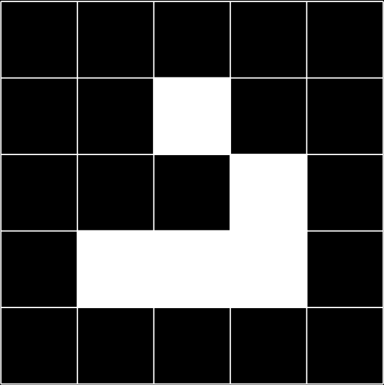
gider start configuration.
        glider = [0 1 0;
                  0 0 1;
                  1 1 1];
game_of_life() needs to be a little modified to save the number of cells in each time step.
n_cells = zeros(Int64,t)
for τ in 1:t
n_cells[τ] = sum(state)
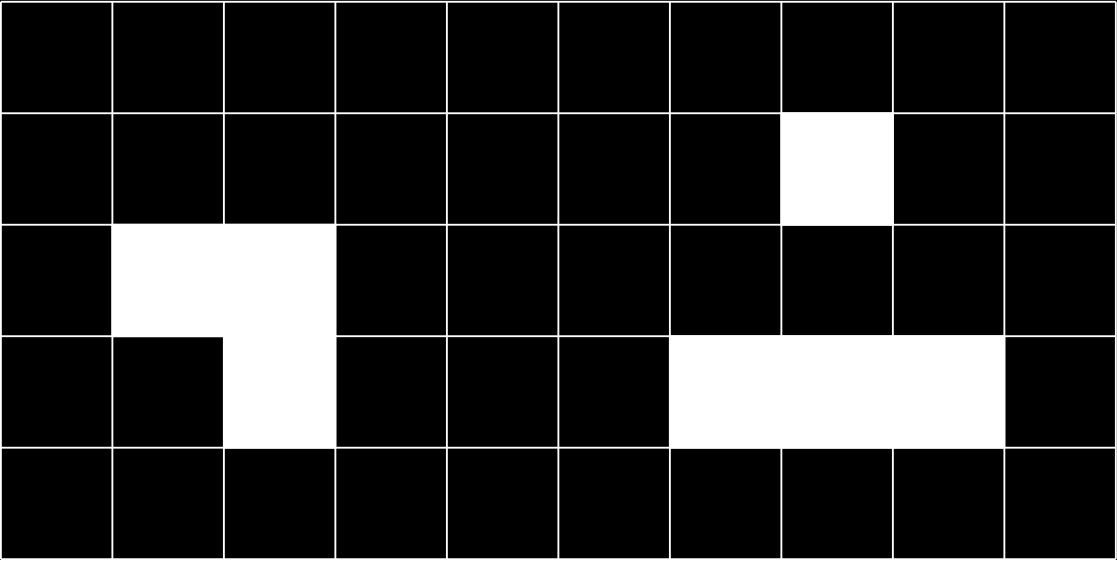
diehard start configuration.
        diehard = [0 0 0 0 0 0 1 0;
                   1 1 0 0 0 0 0 0;
                   0 1 0 0 0 1 1 1];